Tutorial

The goal of this tutorial is to show how to set up and analyse a simulation using the dompap package. After completing this tutorial, you should be able to:

• Set initial positions of particles

• Set initial velocities of particles

• Set the pair potential of the particles

• Set up the integrator (time step, target temperature etc.).

• Equilibrate the simulation

• Make a production run

• Visualise the simulation

• Compute thermodynamic properties of the system (pressure, energy, etc.)

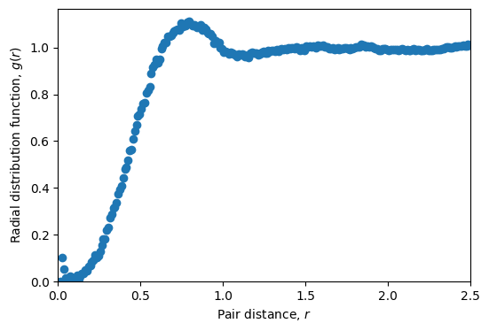
• Compute and plot the radial distribution function.

For other tasks, such as setting up different models, and other analysis you should consult the examples in the documentation.

Introduction

This tutorial will show how to set up, and analyse a simulation. We will simulate a three-dimensional system of particles with harmonic repulsions These are particles that interact with the pair energy

(1)\[\begin{equation} v(r) = (1-r)^2 \end{equation}\]

for \(r<1\) and zero otherwise.

# Imports
import numpy as np
import matplotlib.pyplot as plt
import dompap  # Import the dompap package

First, we need to import the Simulation class from the dompap module, and create an instance of it.

sim = dompap.Simulation()  # Create an instance of the Simulation class

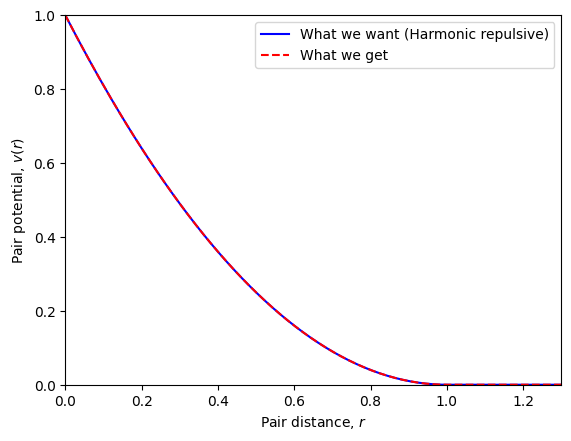
Pair potential

We can set (and plot) the pair potential of the particles of the current simulation object.

# Set pair potential
sim.set_pair_potential(pair_potential_str='(1-r)**2',
                       r_cut=1.0,
                       force_method='neighbor list',
                       energy_method='neighbor list')
sim.set_pair_potential_parameters(sigma=1.0, epsilon=1.0)

# Plot pair potential
plt.figure()
r = np.linspace(0.0, 2, 200)
v_test = (1-r)**2*np.heaviside(1.0-r, 0.5)
plt.plot(r, v_test, 'b-', label='What we want (Harmonic repulsive)')
plt.plot(r, sim.pair_potential(r), 'r--', label='What we get')
plt.xlabel(r'Pair distance, $r$')
plt.ylabel('Pair potential, $v(r)$')
plt.ylim(0, 1)
plt.xlim(0, 1.3)
plt.legend()
plt.show()

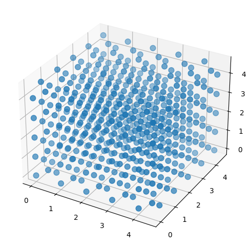
Set initial positions and velocities

Next we set positions into an fcc lattice.

fcc_unit_cell = ([0.0, 0.0, 0.0],
                 [0.5, 0.5, 0.0],
                 [0.5, 0.0, 0.5],
                 [0.0, 0.5, 0.5])
sim.set_positions(unit_cell_coordinates=fcc_unit_cell,
                  cells=(5, 5, 5),
                  lattice_constants=(1.0, 1.0, 1.0))

# Extract positions
x, y, z = sim.positions[:, 0], sim.positions[:, 1], sim.positions[:, 2]

# ... and create a 3d scatter plot
fig = plt.figure(figsize=(6, 6))
ax = fig.add_subplot(111, projection='3d')
ax.scatter(x, y, z, s=60)
plt.show()

Set masses and initial velocities.

sim.set_masses(masses=1.0)
sim.set_random_velocities(temperature=0.1)

Setup \(NVE\) integrator (temperature_damping_time=np.inf) and parameters for neighbour list.

sim.set_integrator(time_step=0.01,
                   target_temperature=0.1,
                   temperature_damping_time=0.1)

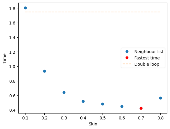
Autotuner

Use autotuner to set algorithm and parameters for most efficient calculations (can also be set manually).

sim = dompap.tools.autotune(sim, verbose=True, plot=True)

Time to update neighbor list (double loop): 81.383 milliseconds
Time to update neighbor list (double loop): 81.898 milliseconds
Time to update neighbor list (double loop): 81.650 milliseconds

Time to update neighbor list (double loop): 82.022 milliseconds

Time to update neighbor list (cell list): 101.183 milliseconds
Time to update neighbor list (cell list): 101.158 milliseconds
Time to update neighbor list (cell list): 101.252 milliseconds

Time to update neighbor list (cell list): 101.667 milliseconds
Fastest method to update neighbor list: double loop
largest_allowed_skin=np.float64(2.5)

Skin | Time per step (ms) | steps/updates
 0.1 | 18.0529             | 100/22 = 4.5
 0.2 | 9.3325             | 100/11 = 9.1
 0.3 | 6.4196             | 100/7 = 14.3
 0.4 | 5.2155             | 100/5 = 20.0
 0.5 | 4.8220             | 100/4 = 25.0
 0.6 | 4.4867             | 100/3 = 33.3
 0.7 | 4.2542             | 100/2 = 50.0
 0.8 | 5.6588             | 100/2 = 50.0
Optimal parameters: skin=0.7
Time to compute forces (double loop, skin=0.7000): 3.146 milliseconds
Time to compute forces (double loop, skin=0.7000): 3.092 milliseconds
Time to compute forces (double loop, skin=0.7000): 3.075 milliseconds
Time to compute forces (double loop, skin=0.7000): 3.130 milliseconds

Time with double loop: 17.4879 milliseconds

Time with double loop single core: 27.8216 milliseconds

Time with vectorized: 25.6580 milliseconds
Fastest method: neighbor list

Run simluation

steps = 40
for step in range(steps):
    sim.step()
    if step % 10 == 0:
        print(f'Energy after {step} steps: {sim.get_potential_energy()}')

Energy after 0 steps: 257.3801019575987
Energy after 10 steps: 259.2203796339139
Energy after 20 steps: 261.93626452482465
Energy after 30 steps: 264.7390883997492

Runtime analysis

r_bins = np.arange(0.01, 2.5, 0.01)
r, rdf = sim.get_radial_distribution_function(r_bins=r_bins)
rdf_evaluations = 1
steps = 1_000
stride = 4
for step in range(steps):
    sim.step()
    if step % stride == 0:
        _, this_rdf = sim.get_radial_distribution_function(r_bins=r_bins)
        rdf += this_rdf
        rdf_evaluations += 1
rdf /= rdf_evaluations + 1

# Plot radial distribution function
plt.figure(figsize=(6, 4))
plt.plot(r, rdf, 'o')
plt.xlabel(r'Pair distance, $r$')
plt.ylabel(r'Radial distribution function, $g(r)$')
plt.xlim(0, 2.5)
plt.ylim(0, None)
plt.savefig('radial_distribution.png', dpi=300, bbox_inches='tight')
plt.show()